DPT
[1]:
# load modules
import os
import numpy as np
import pandas as pd
import pickle

# Plotting imports
import matplotlib
import matplotlib.pyplot as plt

import palantir
import scanpy as sc
findfont: Font family ['Raleway'] not found. Falling back to DejaVu Sans.
findfont: Font family ['Lato'] not found. Falling back to DejaVu Sans.
[3]:
%matplotlib inline
Download data
Anndata objects with all the data and metadata are publically avaiable at: https://s3.amazonaws.com/dp-lab-data-public/palantir/human_cd34_bm_rep[1-3].h5ad. This notebook use replicate 1 (https://s3.amazonaws.com/dp-lab-data-public/palantir/human_cd34_bm_rep1.h5ad) for illustration.
Description of the anndata object is available at https://s3.amazonaws.com/dp-lab-data-public/palantir/readme
Load data
[4]:
# Load the AnnData object
ad = sc.read('annadata/human_cd34_bm_rep1.h5ad')
colors = pd.Series(ad.uns['cluster_colors'])
ct_colors = pd.Series(ad.uns['ct_colors'])
DPT
[5]:
# Set the start / root cell
ad.uns['iroot'] = np.flatnonzero(ad.obs_names == ad.obs['palantir_pseudotime'].idxmin())[0]
[6]:
# PCA, tSNE, diffusion maps and DPT
sc.pp.pca(ad, n_comps=300)
sc.tl.tsne(ad);
sc.pp.neighbors(ad, 50)
sc.tl.diffmap(ad, 10)
sc.tl.dpt(ad, n_dcs=10, n_branchings=3, copy=False)
Note that scikit-learn's randomized PCA might not be exactly reproducible across different computational platforms. For exact reproducibility, choose `svd_solver='arpack'.` This will likely become the Scanpy default in the future.
computing PCA with n_comps = 300
    finished (0:00:04.45)
    and added
    'X_pca', the PCA coordinates (adata.obs)
    'PC1', 'PC2', ..., the loadings (adata.var)
    'pca_variance', the variance / eigenvalues (adata.uns)
    'pca_variance_ratio', the variance ratio (adata.uns)
computing tSNE
    using 'X_pca' with n_pcs = 300
    using the 'MulticoreTSNE' package by Ulyanov (2017)
    finished (0:00:51.46) --> added
    'X_tsne', tSNE coordinates (adata.obsm)
computing neighbors
    using 'X_pca' with n_pcs = 300
    computed neighbors (0:00:00.72)
    computed connectivities (0:00:06.74)
    finished (0:00:00.02) --> added to `.uns['neighbors']`
    'distances', distances for each pair of neighbors
    'connectivities', weighted adjacency matrix
computing Diffusion Maps using n_comps=10(=n_dcs)
        initialized `.distances` `.connectivities`
    computed transitions (0:00:00.04)
    eigenvalues of transition matrix
    [1.         0.9849899  0.97812945 0.9549652  0.9394395  0.92903304
     0.9068288  0.90428394 0.8509435  0.8371804 ]
    finished (0:00:00.25) --> added
    'X_diffmap', diffmap coordinates (adata.obsm)
    'diffmap_evals', eigenvalues of transition matrix (adata.uns)
        initialized `.distances` `.connectivities` `.eigen_values` `.eigen_basis` `.distances_dpt`
computing Diffusion Pseudotime using n_dcs=10
    this uses a hierarchical implementation
        detect 3 branchings
        do not consider groups with less than 57 points for splitting
        group 0 score 1.555689 n_points 5780
        branching 1: split group 0
        group 0 score 1.3113303 n_points 63
        group 1 score 1.6766814 n_points 1196
        group 2 score 1.1366823 n_points 562
        group 3 score 1.6420908 n_points 2799
        branching 2: split group 1
        group 0 score 1.3113303 n_points 63
        group 1 score 0.26748806 n_points 5 (too small)
        group 2 score 1.1366823 n_points 562
        group 3 score 1.6420908 n_points 2799
        group 4 score 1.2083104 n_points 970
        group 5 score 1.333738 n_points 151
        group 6 score 1.0511937 n_points 47 (too small)
        branching 3: split group 3
    finished (0:00:04.93) --> added
    'dpt_pseudotime', the pseudotime (adata.obs)
    'dpt_groups', the branching subgroups of dpt (adata.obs)
    'dpt_order', cell order (adata.obs)
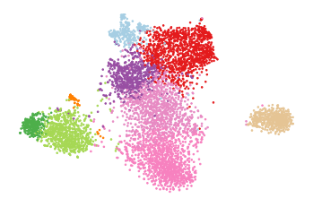
Plot below shows the tSNE map colored using the same color scheme shown in Fig 2
[7]:
plt.scatter(ad.obsm['X_tsne'][:, 0], ad.obsm['X_tsne'][:, 1],
           s=3, color=colors[ad.obs['clusters']])
ax = plt.gca()
ax.set_axis_off()
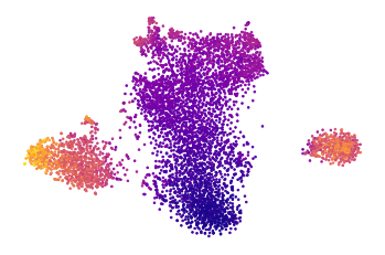
Pseudotime
[8]:
plt.scatter(ad.obsm['X_tsne'][:, 0], ad.obsm['X_tsne'][:, 1],
           s=3, c=ad.obs['dpt_pseudotime'], cmap=matplotlib.cm.plasma)
ax = plt.gca()
ax.set_axis_off()
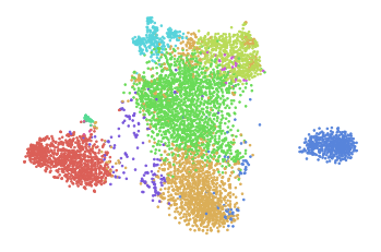
Branches
Branches identified by DPT
[9]:
branches = ad.obs['dpt_groups'].unique()
dpt_colors = matplotlib.colormaps["hls"](range(len(branches)))
dpt_colors = pd.Series([matplotlib.colors.rgb2hex(rgba) for rgba in dpt_colors], index = branches)
[13]:
plt.scatter(ad.obsm['X_tsne'][:, 0], ad.obsm['X_tsne'][:, 1],
           s=3, color=dpt_colors[ad.obs['dpt_groups'].values])
ax = plt.gca()
ax.set_axis_off()
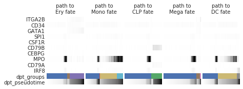
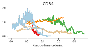
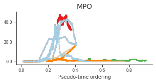
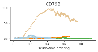
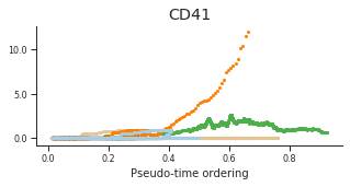
Trends
[14]:
genes = ['CD34', 'MPO', 'IRF8', 'CD79A', 'GATA1', 'ITGA2B'] + \
    ['CD34', 'SPI1', 'MPO', 'GATA1', 'IRF8', 'CD79B', 'CEBPG', 'CSF1R']
genes = list(set(genes))
[15]:
trends = pd.Series()
[16]:
paths = [('Ery', [0, 5, 4]),  # use the category indices instead of the cluster names
         ('Mono', [0, 3, 8, 9]),
         ('CLP', [0, 2]),
         ('Mega', [0, 5, 6]),
         ('DC', [0, 3, 8, 7])]

_, axs = plt.subplots(ncols=len(paths), figsize=(6, 2.5), gridspec_kw={'wspace': 0.05, 'left': 0.11})
plt.subplots_adjust(left=0.05, right=0.98, top=0.82, bottom=0.2)
for ipath, (descr, path) in enumerate(paths):
    _, data = sc.pl.paga_path(
        ad, path, genes,
        show_node_names=False,
        groups_key='dpt_groups',
        ax=axs[ipath],
        n_avg=50,
        show_yticks=True if ipath==0 else False,
        show_colorbar=False,
        color_map='Greys',
        title='path to\n{} fate'.format(descr),
        return_data=True,
        show=False)
    trends[descr] = data
generating colors for dpt_groups using palette
[17]:
from matplotlib.ticker import FormatStrFormatter
[18]:
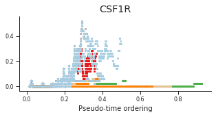
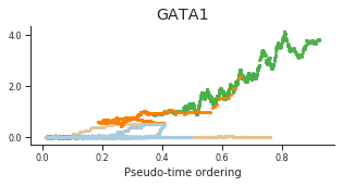
genes = ['CD34', 'MPO',  'CD79B', 'ITGA2B', 'CSF1R', 'GATA1']
labels = ['CD34', 'MPO', 'CD79B', 'CD41', 'CSF1R', 'GATA1']

for gene, label in zip(genes, labels):
    fig = plt.figure(figsize=[5, 2])

    ax = plt.gca()

    for l in trends.keys():
        order = trends[l].distance.sort_values().index

        bins = np.ravel(trends[l].distance[order])
        t = np.ravel(trends[l].loc[order, gene])

        # Plot
        plt.scatter(bins, t, color=ct_colors[l], s=5)


    ax.set_title(label)
    ax.set_xlabel('Pseudo-time ordering', fontsize=10)
    ax.yaxis.set_major_formatter(FormatStrFormatter('%.1f'))
    plt.xticks(fontsize=8)
    plt.yticks(fontsize=8)
[ ]: